
This blog post is a successor to the one about escape analysis in PyPy's JIT. The examples from there will be continued here. This post is a bit science-fictiony. The algorithm that PyPy currently uses is significantly more complex and much harder than the one that is described here. The resulting behaviour is very similar, however, so we will use the simpler version (and we might switch to that at some point in the actual implementation).
In the last blog post we described how escape analysis can be used to remove many of the allocations of short-lived objects and many of the type dispatches that are present in a non-optimized trace. In this post we will improve the optimization to also handle more cases.
To understand some more what the optimization described in the last blog post can achieve, look at the following figure:

The figure shows a trace before optimization, together with the lifetime of various kinds of objects created in the trace. It is executed from top to bottom. At the bottom, a jump is used to execute the same loop another time. For clarity, the figure shows two iterations of the loop. The loop is executed until one of the guards in the trace fails, and the execution is aborted.
Some of the operations within this trace are new operations, which each create a new instance of some class. These instances are used for a while, e.g. by calling methods on them, reading and writing their fields. Some of these instances escape, which means that they are stored in some globally accessible place or are passed into a function.
Together with the new operations, the figure shows the lifetimes of the created objects. Objects in category 1 live for a while, and are then just not used any more. The creation of these objects is removed by the optimization described in the last blog post.
Objects in category 2 live for a while and then escape. The optimization of the last post deals with them too: the new that creates them and the field accesses are deferred, until the point where the object escapes.
The objects in category 3 and 4 are in principle like the objects in category 1 and 2. They are created, live for a while, but are then passed as an argument to the jump operation. In the next iteration they can either die (category 3) or escape (category 4).
The optimization of the last post considered the passing of an object along a jump to be equivalent to escaping. It was thus treating objects in category 3 and 4 like those in category 2.
The improved optimization described in this post will make it possible to deal better with objects in category 3 and 4. This will have two consequences: on the one hand, more allocations are removed from the trace (which is clearly good). As a side-effect of this, the traces will also be type-specialized.
Optimizing Across the Jump
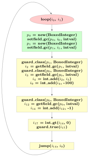
Let's look at the final trace obtained in the last post for the example loop. The final trace was much better than the original one, because many allocations were removed from it. However, it also still contained allocations:

The two new BoxedIntegers stored in p15 and p10 are passed into the next iteration of the loop. The next iteration will check that they are indeed BoxedIntegers, read their intval fields and then not use them any more. Thus those instances are in category 3.
In its current state the loop allocates two BoxedIntegers at the end of every iteration, that then die very quickly in the next iteration. In addition, the type checks at the start of the loop are superfluous, at least after the first iteration.
The reason why we cannot optimize the remaining allocations away is because their lifetime crosses the jump. To improve the situation, a little trick is needed. The trace above represents a loop, i.e. the jump at the end jumps to the beginning. Where in the loop the jump occurs is arbitrary, since the loop can only be left via failing guards anyway. Therefore it does not change the semantics of the loop to put the jump at another point into the trace and we can move the jump operation just above the allocation of the objects that appear in the current jump. This needs some care, because the arguments to jump are all currently live variables, thus they need to be adapted.
If we do that for our example trace above, the trace looks like this:
Now the lifetime of the remaining allocations no longer crosses the jump, and we can run our escape analysis a second time, to get the following trace:

This result is now really good. The code performs the same operations than the original code, but using direct CPU arithmetic and no boxing, as opposed to the original version which used dynamic dispatching and boxing.
Looking at the final trace it is also completely clear that specialization has happened. The trace corresponds to the situation in which the trace was originally recorded, which happened to be a loop where BoxedIntegers were used. The now resulting loop does not refer to the BoxedInteger class at all any more, but it still has the same behaviour. If the original loop had used BoxedFloats, the final loop would use float_* operations everywhere instead (or even be very different, if the object model had user-defined classes).
Entering the Loop
The approach of placing the jump at some other point in the loop leads to one additional complication that we glossed over so far. The beginning of the original loop corresponds to a point in the original program, namely the while loop in the function f from the last post.
Now recall that in a VM that uses a tracing JIT, all programs start by being interpreted. This means that when f is executed by the interpreter, it is easy to go from the interpreter to the first version of the compiled loop. After the jump is moved and the escape analysis optimization is applied a second time, this is no longer easily possible. In particular, the new loop expects two integers as input arguments, while the old one expected two instances.
To make it possible to enter the loop directly from the intepreter, there needs to be some additional code that enters the loop by taking as input arguments what is available to the interpreter, i.e. two instances. This additional code corresponds to one iteration of the loop, which is thus peeled off:

Summary
The optimization described in this post can be used to optimize away allocations in category 3 and improve allocations in category 4, by deferring them until they are no longer avoidable. A side-effect of these optimizations is also that the optimized loops are specialized for the types of the variables that are used inside them.
1 comment:
Interesting, like the previous post. Keep 'em coming. :)
Post a Comment